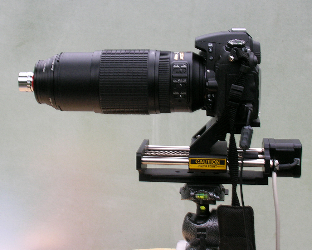
I had to create scans of a small flex PCB to capture more details than a flat scanner could give me. Of course, this task turned out harder than I imagined. I already had a good camera, but I was lacking a good macro lens. Buying one turned out to be hard because the highest magnification ratios on most macro lenses are 1:1. The better ones are, of course, pricier.

Adapting Microscope Objectives for Macrophotography

After browsing some extreme macrophotography forums, I discovered that some people use microscope objectives with their cameras.

An infinite microscope (silver element on the left) lens mounted on a camera. Source: Thorninger.com

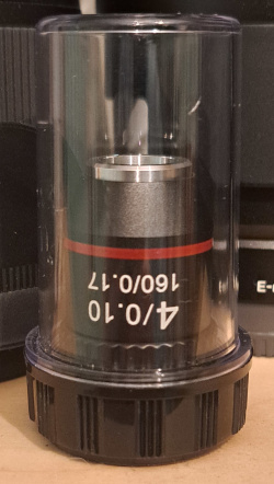
Those microscope objectives are divided into two groups: infinity-corrected and non-infinity-corrected. What does this mean? The non-infinity-corrected objective focuses the captured image on a plane some distance after the objective. The infinity-corrected objective collimates the captured light into a parallel beam. The second type is useful if you need to Fourier transform the image by transparency masks or do other fancy scientific image transformations. Filtering light is easier if you work with a parallel beam. To use this type of objective in macrophotography, you need an additional lens to focus the parallel beam to an image on the sensor plane.

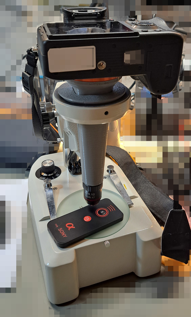
The first type of microscope objective can be used directly with your interchangeable lens camera. The only thing you need is an extension tube, which can be 3D printed in an hour. I found a great Thingiverse repository that contains extension tubes for microscopic objectives with various camera mounts. Together with the cheapest 4X non-infinity-corrected, achromatic microscope objective gives decent results.

Cheap AliExpress microscope objective

       

My setup mounted on an inspection microscope stand to precisely control focus.

Taking Pictures

And now the hardest part. I spent a few days taking pictures of different PCBs to stitch them into a bigger picture. Messing up this step will lead to more errors later. My advice is to fix your camera at a distance at which your object is in focus and then move your object in a specific way. Scan your object in a linear way, incrementing only one dimension (X or Y) at a time, as illustrated in the image below. Your next picture should overlap with your previous one by 30% - 50%. If you are using a full-frame camera, try to use it in crop mode or just make smaller movements. This way, you will be using only the sharpest and least distorted image of your microscope lens. And remember, good and uniform lighting is everything.

Image Processing

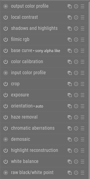
You can use JPEGs straight out of the camera, but I like to process my RAW files in darktable. It can be useful to set the correct exposure and contrast at this stage because, after stitching, changing those parameters can further enhance seams on the final image. Whatever you do, do not reduce noise or add noise in highlight correction because this will reduce the alignment coefficients in Hugin. I usually further crop the images to remove portions with the biggest distortions. You can export the images in JPEG with 98% quality to reduce file size. I noticed that usually, the cheap microscope lens is the limiting factor, and you don’t need high pixel quality/density.

Example darktable stack that I'm using

Stitching with Hugin

Hugin is an image software toolbox that can be used for various image manipulation and correction. Such elasticity comes at a cost of complexity.

The first thing that you have to do to start stitching microscope images after running Hugin - Panorama Stitcher is to change the interface to expert by clicking Interface->Expert. Next, in File->Preferences under the Control Point Detector tab, click New and add once again Hugin’s CPFind but with --linearmatch --linearmatchlen=2 -o %o %s as arguments. The value in the field Program: should be copied from the Hugin’s CPFind entry because it depends on where you have Hugin installed. This option will match images to their neighbors, instead of matching every image with every image, drastically reducing computing time for large image sets and improving accuracy.

Then the workflow is as follows:

1. Add images by clicking Add images....
2. Select all images from the scan.
3. Set Lens type: Normal (rectilinear).
4. Set HFOV (v) to 10 degrees.
5. Set Focal length multiplier to 1.
6. Choose your created Hugin CPFind with linearmatch arguments script from the Feature Matching Settings: list and click Create control points.
7. Choose Custom parameters from Optimize, Geometric: list.
8. Change the view to the Optimiser tab.
9. Right-click on Yaw (y) and click Unselect all. Do this for other columns as well.
10. Right-click on X (TrX) and click Select all. Do this also for Y (TrY) and Roll (r) (check roll only if images got flipped by your camera or you rotated your object).

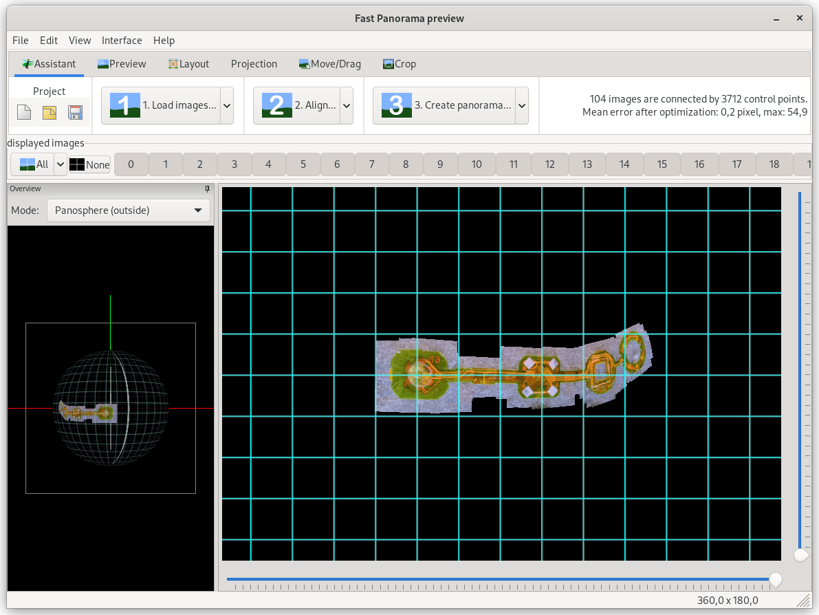
11. Click on Optimize now!. If you see a result similar to that below, you are good. If the values are all zeros or in the order of thousands, you should capture your images once again. But this time put more effort into that. ;P

    Optimiser run finished.
    Results:
     average control point distance: 0.209935
     standard deviation: 1.102026
     maximum: 54.850377
        
    Apply the changes?
    

12. Click on Preview panorama (OpenGL) - ninth button on the top bar with the GL letters.
13. See if your images are semi-aligned and create a continuous image. They can be a little misplaced. Again, if the images are not visible or are not aligned, you should start over and take better images. It will be faster than trying to align your images by hand.
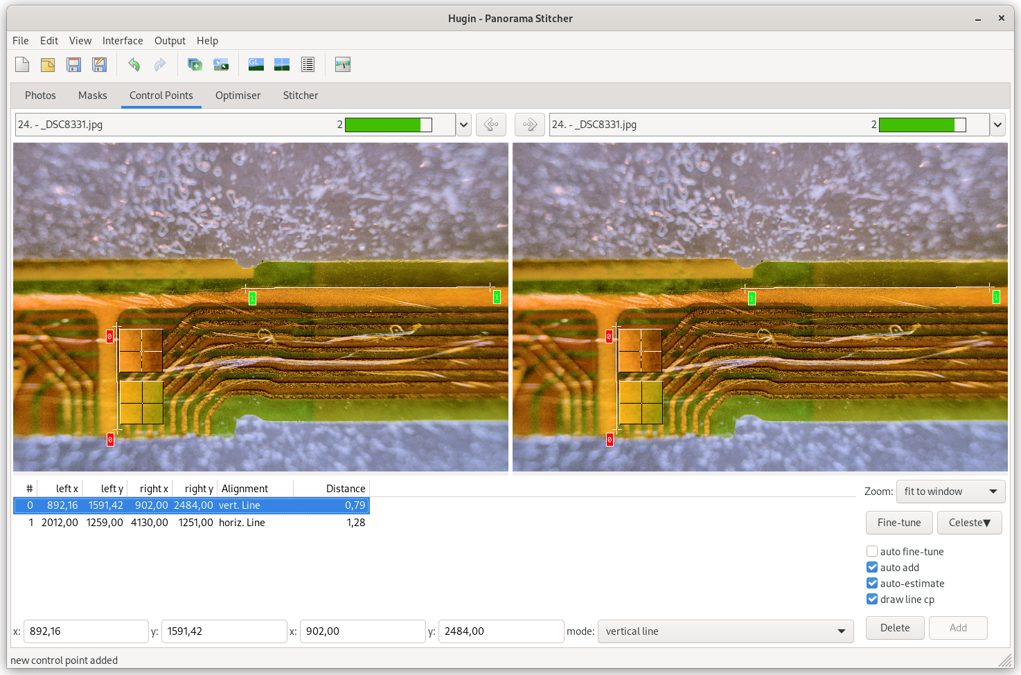
14. Now return to the previous Hugin window and open the Control Points tab.
15. Select the first image on the left window and on the right window.
16. Using arrows between the image name lists, change images and pause on those that have long vertical or horizontal elements.
17. By left-clicking on the left image, select the beginning of the horizontal or vertical element. And then on the right image, click on the end of that element. Uncheck auto fine-tune if the points jump around. Repeat this step for as many images as you like.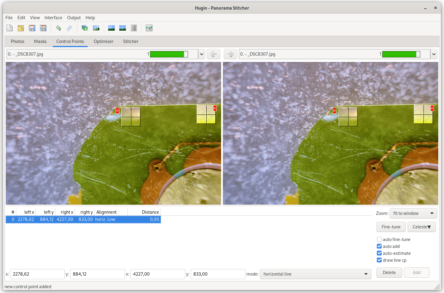
18. Click Optimize now! in the Optimiser tab again.
19. Switch your view to Fast Panorama preview again.
20. Click on Move/Drag tab.
21. Move your PCB to the center of the view or click the Centre button on the top left.
22. Switch the tab to Projection.
23. Choose Rectilinear from the top list.
24. Click on the Fit button on the top left.
25. Choose Mosaic plane in the Mode: list. If you get a prompt with Should the Tpy and Tpp parameters reset to zero?, click Yes.
26. Return to the Hugin main window to the Photos tab.
27. Choose Hugin's CPFind (prealigned) in the Feature Matching Settings: list.
28. Click Create control points.
29. Return to the Optimiser tab and click Optimize now!.
30. Repeat steps 19-25.
31. Click on Show control points - eleventh button from the top left.
32. Click on the Distance column and sort your points in descending distance order.
33. Remove the top ones. You can do it automatically, but it is better to inspect them one by one and do it by hand. If you have Fast Panorama preview open, the selected points will show up in that window. Do not remove your horizontal or vertical line points.
34. Click Optimize now! again.
35. See in Fast Panorama preview if your image didn’t blow up. If yes, congratulations, you can capture your images again or add more control points by hand and try from step 18.
36. If everything looks good, go into the Optimiser tab and right-clicking on columns Z (TrZ), Hfov (v), and Select all. Select the Roll (r) column also if you didn’t do it earlier.
37. Click Optimize now!.
38. The worst step. Return to previous steps and experiment if you are not satisfied with the results.
39. In Fast Panorama preview, in the Crop tab, crop your image using the white bars visible on the image.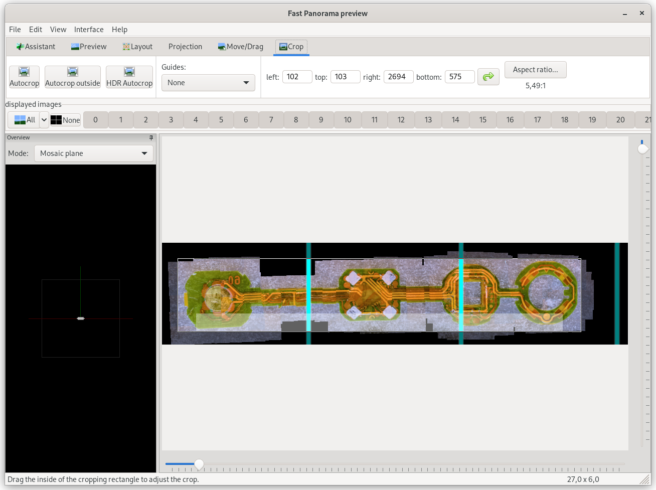
40. Finally, go to the Stitcher tab in the main Hugin window and click on Calculate Optimal Size. The size of the output image will depend on the resolution of the input images, the object size, crop, and optimized field of view.
41. Select the first three checkboxes in the Panorama Outputs section and choose the desired output file format.
42. Click on Stitch! button on the right bottom.

Three image files should be created. Review them and choose the best one. If you are not satisfied with your result, take better photos or fiddle around with control points in Hugin.

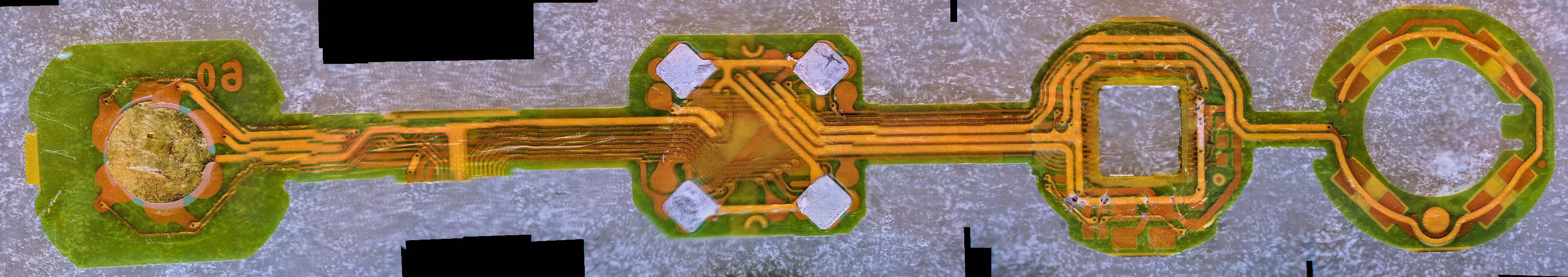
If you stumble on any errors during image stitching, it will probably be an image duplication or the images are not a part of the same set/object. And if the output image has some blurs or shifts (like the one in the image above), try adding more control points between similar images in the Control Points tab in Hugin’s main window.

Resources on which I Based

• [1] https://thorninger.com/eng/extrememacro2.html
• [2] https://patdavid.net/2013/01/focus-stacking-macro-photos-enfuse
• [3] https://derekdvleung.wixsite.com/main/post/stitching-microscope-images-using-hugin